Data Preprocessing

Now as we have visualized some of the data in the dataset.Lets gets ready for training our classifier on but lets wait.we need to pre-process our data so that our model is easy to train and results are much better .

we need to normalize our images because of varying intensities of pixel values.We know that pixel value ranges from 0-255.and images which we are dealing with are greyscaled images i.e most of them would e having pixel values as 0 or 255.Normalization basically compresses these varying intensities of pixel values .

Train Test Split

Now lets split our train test data and ensure reproducibility by seeding.As data provided to us is already split into train and test .Just put a random seed and start training the Model

# Now lets set a random seed so that our results are reproducible
seed = 5 
np.random.seed(seed)

Convolutional Neural Networks

Convolutional Neural Networks are very similar to ordinary Neural Networks.Each neuron receives some inputs, performs a dot product and optionally follows it with a non-linearity.

We could also use a traditional Neural Network like the feed forward neural network . But just imagine the situation. < the first layer of our Network would be a input layer consisting of our feature vector(input vectors).In our case feature vectors are the raw image pixels.28x28 pixels i.e 784 raw pixel values .and if we would be having a colored image of RGB channel this would result in 2352 length feature vector.And our network would be having multiple hidden layers ,this even worsens the scenario.

Convolutional Neural Networks on the other hand exploits spatial relationship between the pixel values.Unlike

Model Building

We woluld be using Keras and Tensorflow for Building Convolutional Neural Networks.

Preprocessing for Keras

For keras some preprocessing is required for feeding our data into model.we need to put our input images into a a particular format.images we have are currently in form [height,width,channel] but keras need it input in a format [no of samples,height,width,channels]

 
  # reshapes values into [no of samples,height,width,channel] 
  images = Digits_train.values.reshape(-1,28,28,1) 
  # no of samples = 1 indicates that we haven't chosen our size and we can choose any random no of samples for training 
  

Encoding Labels

We would be evaluating our model's perfomance on a multiclass classification metric. i.e cross entropy with logits keras has this evaluation metric predefined.but it requires labels to one-hot-encoded. So lets convert our labels into one hot encoded vectors.

 
from keras.utils.np_utils import to_categorical 
labels = to_categorical(labels) 

Lets define our models

 
from keras.models import Sequential 
from keras.layers import Dense,Conv2D,MaxPool2D,Flatten,Dropout 
from keras.activations import relu,softmax 
def CNN_model(): 
  model = Sequential() 
  model.add(Conv2D(64,(3,3),padding= 'Same',activation ='relu', input_shape = (28,28,1))) model.add(MaxPool2D()) 
  model.add(Conv2D(32,(3,3),padding = 'Same',activation ='relu', input_shape = (28,28,1))) model.add(MaxPool2D()) 
  model.add(Conv2D(16,(3,3),padding = 'Same',activation
  ='relu', input_shape = (28,28,1))) 
  model.add(MaxPool2D()) 
  model.add(Dropout(0.5)) 
  model.add(Flatten()) 
  model.add(Dense(128)) 
  model.add(Dropout(0.5)) 
  model.add(Dense(10,activation = "softmax")) 
  return model 

 
CNN_model().summary() 

    ________________________________________________________________
Layer (type)                 Output Shape              Param #
=================================================================
conv2d_1 (Conv2D)            (None, 28, 28, 64)        640
_________________________________________________________________
max_pooling2d_1 (MaxPooling2 (None, 14, 14, 64)        0
_________________________________________________________________
conv2d_2 (Conv2D)            (None, 14, 14, 32)        18464
_________________________________________________________________
max_pooling2d_2 (MaxPooling2 (None, 7, 7, 32)          0
_________________________________________________________________
conv2d_3 (Conv2D)            (None, 7, 7, 16)          4624
_________________________________________________________________
max_pooling2d_3 (MaxPooling2 (None, 3, 3, 16)          0
_________________________________________________________________
dropout_1 (Dropout)          (None, 3, 3, 16)          0
_________________________________________________________________
flatten_1 (Flatten)          (None, 144)               0
_________________________________________________________________
dense_1 (Dense)              (None, 128)               18560
_________________________________________________________________
dropout_2 (Dropout)          (None, 128)               0
_________________________________________________________________
dense_2 (Dense)              (None, 10)                1290
=================================================================
Total params: 43,578
Trainable params: 43,578
Non-trainable params: 0
_________________________________________________________________

Compile and Run our model

Since we have now defined our model , we will just need to define the loss function evaluation metrics and epochs.

 
model = CNN_model() 
model.compile(loss='categorical_crossentropy',optimizer='adam',metrics=['accuracy'])

 
history = model.fit(img,labels,epochs=10, batch_size=50,validation_split=0.2,verbose=2,shuffle=False) 

Train on 33600 samples, validate on 8400 samples
Epoch 1/10
 - 65s - loss: 0.6216 - acc: 0.7924 - val_loss: 0.1098 - val_acc: 0.9671
Epoch 2/10
 - 67s - loss: 0.2327 - acc: 0.9252 - val_loss: 0.0763 - val_acc: 0.9777
Epoch 3/10
 - 65s - loss: 0.1782 - acc: 0.9452 - val_loss: 0.0641 - val_acc: 0.9804
Epoch 4/10
 - 66s - loss: 0.1494 - acc: 0.9550 - val_loss: 0.0524 - val_acc: 0.9837
Epoch 5/10
 - 65s - loss: 0.1321 - acc: 0.9583 - val_loss: 0.0507 - val_acc: 0.9850
Epoch 6/10
 - 66s - loss: 0.1202 - acc: 0.9632 - val_loss: 0.0513 - val_acc: 0.9846
Epoch 7/10
 - 66s - loss: 0.1157 - acc: 0.9640 - val_loss: 0.0455 - val_acc: 0.9876
Epoch 8/10
 - 66s - loss: 0.1042 - acc: 0.9676 - val_loss: 0.0439 - val_acc: 0.9865
Epoch 9/10
 - 67s - loss: 0.0995 - acc: 0.9693 - val_loss: 0.0404 - val_acc: 0.9882
Epoch 10/10
 - 65s - loss: 0.0908 - acc: 0.9713 - val_loss: 0.0383 - val_acc: 0.9886

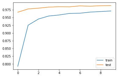
we have trained our model on 10 epochs.20 % data has been set aside for validation.

plt.plot(history.history['acc'], label='train') 
plt.plot(history.history['val_acc'], label='test') 
plt.legend() 

The above graph clearly indicates how out model performs both on the test set and validation set.we have used 20% of our training data as our validation set

Clearly our model performs well on the train set with accuracy of about 97.13% and on our validation set 98.86%>.Overfitting occurs when accuracy on the train data is higher than the validation dataset or the test dataset

Predictions

Now we will check our predictions on the testing dataset .lets verify by classifying one image from the dataset as well as plotting it.

But before predicting our output we need to transform our test data into format data and do some preprocessing i.e normalizing pixel intensities.

 
Digits_test = Digits_test/255.0 
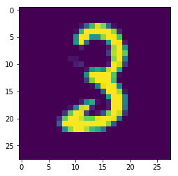
Digits_test = Digits_test.values.reshape(-1,28,28,1) 

plt.imshow(Digits_test[4][:,:,0]) 

Clearly the image shows that the image is that of number 3.Lets verify it by predicting it

 
              label = model.predict(Digits_test[4].reshape(-1,28,28,1))
               print label 
               

    array([[1.35892244e-11, 6.63674093e-09, 1.89812010e-06, 9.99997854e-01,
        5.45060850e-13, 7.55617506e-08, 2.06700043e-12, 1.03831745e-07,
        1.64455578e-08, 2.63139732e-09]], dtype=float32)

In the last layer of Convolutional Neural Networks ,we have used a softmax classifier.It output probabilities of various classes i.e Ten probabilities corresponding to digits 0-9.If you observe carefully the index 3 of the array has the probability 0.99 which is the number 3 class of our dataset.

Check here for the MNIST Recognition App